Development of a Cointegrated Pairs Trading Strategy
Practical implementation of a simple cointegrated pairs trading strategy using equities
Introduction
Pairs trading is a market-neutral trading strategy that allows traders to profit from any market regime. It can also be called statistical arbitrage or convergence trading.
The theory underlying Pairs Trading goes that the prices of two companies in the same sector will diverge due to certain events affecting one of them. The idea is to simultaneously long and short these two assets while they diverge and exit when they revert to the mean. This translates to believing that their long-running spread will remain in equilibrium despite eventual short-term price disruptions affecting one of the two companies’ price because both companies will likely be exposed to similar market factors.
Cointegration forms the basis of pairs trading. Let’s introduce it with its mathematical definition:
If there exists a stationary linear combination of two or more non-stationary variables, the variables combined are said to be cointegrated.
In other words, two random processes are said to be cointegrated while neither one hovers around a constant mean, but some combination of them does.
In a cointegrated pairs trading strategy, we will need to know two main factors: the hedge-ratio (β) and the residuals (εₜ). These two are obtained by carrying out a linear regression of the two assets.
For the linear combination, Ordinary Least Squares (OLS) will be used. Let’s suppose we have two cointegrated stocks {yₜ} and {xₜ} with the following cointegrating relationship: yₜ= βxₜ + εₜ
The relationship would mean that {yₜ} tends to be priced {β} times as high as {xₜ}. The hedge-ratio will be used to know how many units of each pair to long or short when carrying out a pairs trade.
The further the OLS Residuals move from the mean, the more divergence between both variables, and hence the more likely they will revert to the mean — that’s what mean reversion is about, upward moves are to be followed by downward moves (to the mean) and vice versa.
The residuals from the OLS will be used for the trade signals generation. If the two assets are cointegrated, the residuals should behave like a stationary process. One of the ways to test for stationarity is to perform the Augmented Dickey-Fuller (ADF) test. The null hypothesis we want to reject consists in the presence of a unit root, which could cause unpredictable results (the series is a random process). When the ADF is applied to the residuals of a linear combination it’s named Cointegrated Augmented Dickey-Fuller (CADF).
The following chart illustrates two cointegrated Random Walks (RW#1 and RW#2) simulating a dummy pairs trading strategy (later on we will be using real assets). At first sight, we can observe that the OLS residuals tend to revert to a constant mean of ~0.

The p-value from the CADF is 0.01, providing evidence that we can reject the null hypothesis of a unit root at the 1% level and conclude that we have a stationary series and hence a cointegrated pair. In other words, we can be 99% confident that the resulting series (OLS Residuals) obtained from the linear combination of RW#1 and RW#2 is stationary. Therefore, the two main time series are most likely cointegrated for the time window analyzed.
Using RW#1 as the independent variable in the regression we get a β of 0.81, so we would have to trade 0.81 units of RW#2 for every 1 unit of RW#1.
Our dummy strategy had 2 pair trades using the following logic:
- OLS Residuals > +10: short RW#1 and long RW#2
- OLS Residuals < -10: Long RW#1 and short RW#2
- OLS Residuals cross over/under 0: exit
Using static numbers such as +10 or -10 as the threshold for entering trades is not recommended. Later on, we will calculate a moving Z-Score by normalizing the deviation of the spread between the OLS Residuals and the mean. This way we won’t be using static numbers that depend on the particular asset but rather standard deviations, which is a more useful approach if we plan to construct a portfolio with multiple pair trading strategies.
Now that we know the basics, let’s create a pairs trading strategy using real assets.
Developing a Cointegrated Pairs Trading Strategy
The assets to be used are ADBE and MSFT from 2005 to 2020. Both are in the tech sector and their prices will likely be influenced by common market factors.

It’s important to pay attention to which asset do we choose for the dependent and independent variables when carrying out the OLS because switching variables will lead to different hedge-ratios and residuals. For this strategy, ADBE will be selected as the independent variable and MSFT as the dependent one.
If we create a scatter plot of their prices, we can see that the relationship is linear, showing a strong positive correlation.
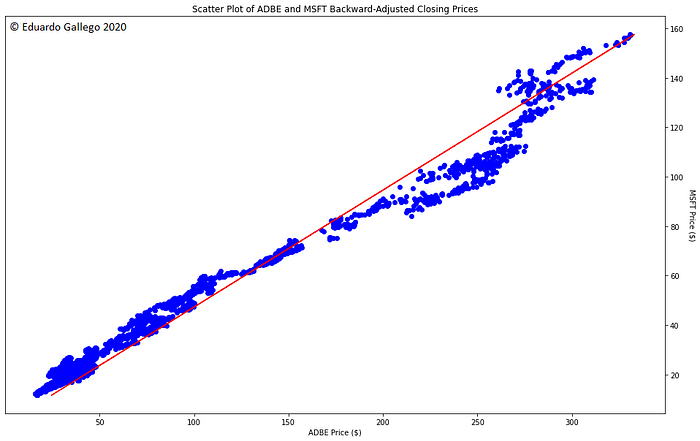
By performing a linear regression between the two assets we get the hedge-ratio and residuals. The hedge-ratio happens to be 2.66, so for every 1 unit of ADBE, we will trade 2.66 of MSFT.
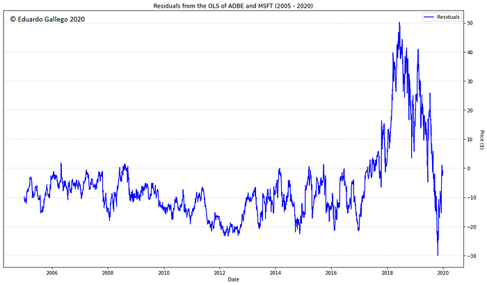
At first glance, the residuals series look like it possesses some stationary behavior. Let’s confirm by carrying out the CADF test.
CADF:
(-3.3872632367838076,
0.011400806292377101,
0,
3774,
{
'1%': -3.4320839039156588,
'5%': -2.8623061432691532,
'10%': -2.567177828379207
},
13274.615166879757)
Given that the test statistic of -3.38 is lower than the 5% level, we can say that there’s enough evidence to reject the null hypothesis of the presence of a unit root.
To generate trading signals from the spread of the linear combination, we will calculate a rolling Z-Score with a period of 100 days.
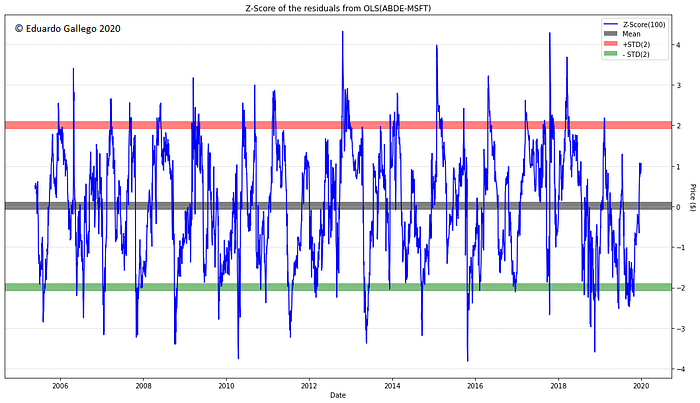
The logic for this strategy is very straight forward:
- Only one pair-trade open at a time.
- $10,000 worth of shares per asset per trade.
- Z-Score < -2STD = Long the spread = Long ADBE and Short MSFT.
- Z-Score > +2STD = Short the spread = Short ADBE and Long MSFT.
- Z-Score crosses over/under the Mean (0) = Exit the trade.
Before looking at the results, it’s worth mentioning that this strategy contains lookahead bias, the OLS and the CADF were calculated over the entire dataset. It should be developed in-sample first and then tested out-of-sample with the values obtained in-sample. But this is outside of the scope of this post, I will dedicate an entire blog post to strategy development and validation shortly.
Results
Net profit: $44,000
Annual return: 16.2%
Profit factor: 2.16
Percent winning: 64.8%
Max Drawdown: 13%
Sharpe ratio: 0.88
Avg trade profit: $500

Final thoughts and practical considerations
The purpose of this post was to keep things simple for the reader to understand cointegration in the context of pairs trading and how to implement a basic trading strategy around it.
Like I mentioned earlier, the strategy hasn’t been optimized or validated whatsoever, and no money or risk management techniques were implemented. Therefore, I don’t recommend trading this live until the corresponding strategy validation tests have been analyzed.
One last thing to consider is that cointegrations, as well as correlations, are not intended to last forever. Rigorous out-of-sample analysis and hedge-ratio checks are recommended from time to time. Black swans and external factors may cause one asset to move way more than it’s expected to, potentially causing the cointegration relationship to break. Having the assets fundamentally related will not guarantee the strategy to work forever but will help to improve the robustness of the strategy.